Some Intuition Behind Double Descent

\( \def\R{\mathbb{R}} \)

2/13/2025

Given a train dataset, what size model will best fit the test distribution? Most intro classes will tell you to pick a medium-sized model following the bias-variance trade-off. Though larger models can represent more complex functions, they may overfit to noise in the training data and get high test error (low bias, high variance). On the other hand, smaller models may underfit the training data and get high training error (high bias, low variance). Figure 1, left captures this intuition. However, anybody practicing machine learning knows that larger models are better. In fact, we spend billions of dollars to train the largest models possible.

Doesn't this defy the bias-variance trade-off? In fact, the bias-variance trade-off is a myth. For sufficiently large model size, referred to as the "overparameterized" regime, the test error can actually start decreasing again! This phenomenon is known as double descent, plotted in Figure 1, right. It can be observed in many settings (Belkin et al, 2018), most notably deep neural networks (Nakkiran et al, 2019). Though this phenomenon has driven empirical progress in machine learning, it is rarely taught in machine learning classes, and students may walk away with the incorrect impression that larger models always overfit.

Why do larger models not overfit? After a lot of work, people found that double descent surprisingly occurs even for plain old linear regression. In the underparameterized regime, one finds that increasing the number of parameters starts overfitting to the noise in the training data. In fact, when the number of parameters is equal to the number of training samples, exactly one model perfectly fits the training data; this solution gets catastrophic test error. In the overparameterized regime, there are many models that perfectly fit the training data, many of which poorly generalize. The magic happens in selecting the minimum norm solution: this particular solution generalizes quite well to the test set, representing an important inductive bias. Interestingly, standard gradient descent is known to converge to the minimum norm solution, showing how optimization interacts with the overparameterized parameter space.

In this post, we will walk through two linear regression settings that exhibit double descent, following the excellent work of Hastie et al, 2019. The first setting will be simpler (ordinary least squares) and the second setting will be a more faithful replication of the double descent phenomenon (latent space features). This post is intended to be an accessible description of the key results, please refer to the original work for more general theorems and the actual proofs!

Standard Linear Regression

Consider the standard linear regression setting where we have $n$ points $(x_i, y_i) \in \R^d \times \R$ for $i \in [n]$, alternatively written as $X \in \R^{n \times p}$ and $y \in \R^n$. We know the outputs are given by $y_i = X\beta^* + \epsilon_i$ for some $\beta^* \in \R^p$ where the inputs are Gaussian $x_i \sim \mathcal{N}(0, \frac{1}{d}I_d)$ and the noise is Gaussian $\epsilon_i \sim \mathcal{N}(0, \sigma^2)$. Given a dataset of $n$ points, we want to find $\beta \in \R^p$ that minimizes the squared loss $||X\beta - y||_2^2$.

In the underparameterized regime ($n < p$), there is a unique solution that minimizes the loss over the training data. This solution is given by the least squares solution

\begin{aligned} \beta &= (X^{\top}X)^{-1}X^{\top}y & \text{[underparameterized solution]} \end{aligned}

In the overparameterized regime ($n > p$), there are many solutions that perfectly fit the training data. Gradient descent (with sufficiently small step size) will provably converge to the solution with the minimum norm. The minimum norm solution is also given by the limit of ridge regression as the weight norm penalty approaches zero. As such, we will use this specific solution to the training data to measure the error of an overparameterized model. The minimum norm solution can be explicitly written as $\beta = (X^{\top}X)^{\dagger}X^{\top}y$ where $\dagger$ denotes the Moore-Penrose pseudoinverse. Since $X^{\top}X$ is full rank in the overparameterized regime, we can rewrite this as

\begin{aligned} \beta &= X^{\top}(XX^{\top})^{\dagger}y & \text{[overparameterized solution]} \end{aligned}

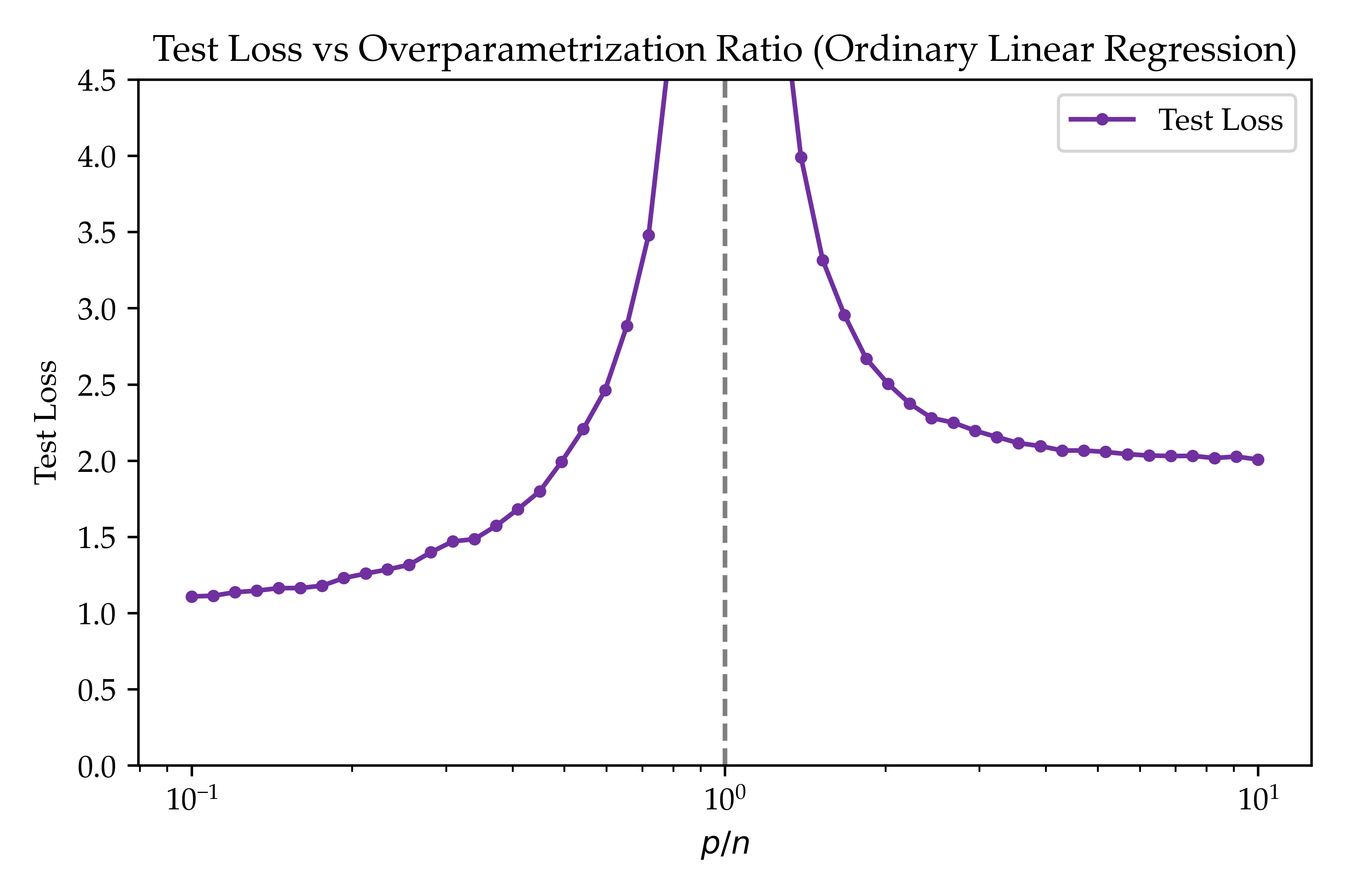
We can now compute the training error of the underparameterized and overparameterized models. In the paper, the authors are able to derive analytic formulas for the error of the models for $n,p \to \infty$ while keeping the ratio $p/n$ fixed. To keep a simpler picture, we simply plot the error as a function of $p/n$ for a fixed (large) $n$ for $\sigma = 1$ in Figure 2. As discussed, when we enter the overparameterized regime, the training error magically starts decreasing! This shows that the double descent phenomenon is not specific to neural networks, giving further insight into why it occurs.

Latent Space Features

The above setting is kind of magical thanks to its simplicity. However, it is missing some important aspects of double descent in practice. Specifically, the optimal solution lies in the underparameterized regime, not the overparameterized regime. This may be because the label generation process changes as we increase the number of parameters, potentially becoming more difficult for larger values of $p$. To address this, we will construct a latent space of fixed dimension $d$ where we sample latents $z_i \sim \mathcal{N}(0, I_d)$. Then, we generate outputs and inputs as

\begin{aligned} y_i &= \theta^{\top}z_i + \xi_i \qquad\qquad x_i = Wz_i + u_i \end{aligned}

for $\theta \in \R^d$, $W \in \R^{d \times p}$, $\xi_i \sim \mathcal{N}(0, \sigma_{\xi}^2)$, and $u_i \sim \mathcal{N}(0, I_p)$. In this model, the (noisy) label is fully defined by the latent (by weight $\theta$) and the inputs can be interpreted as "random features" produced by the latent (by weight $W$).

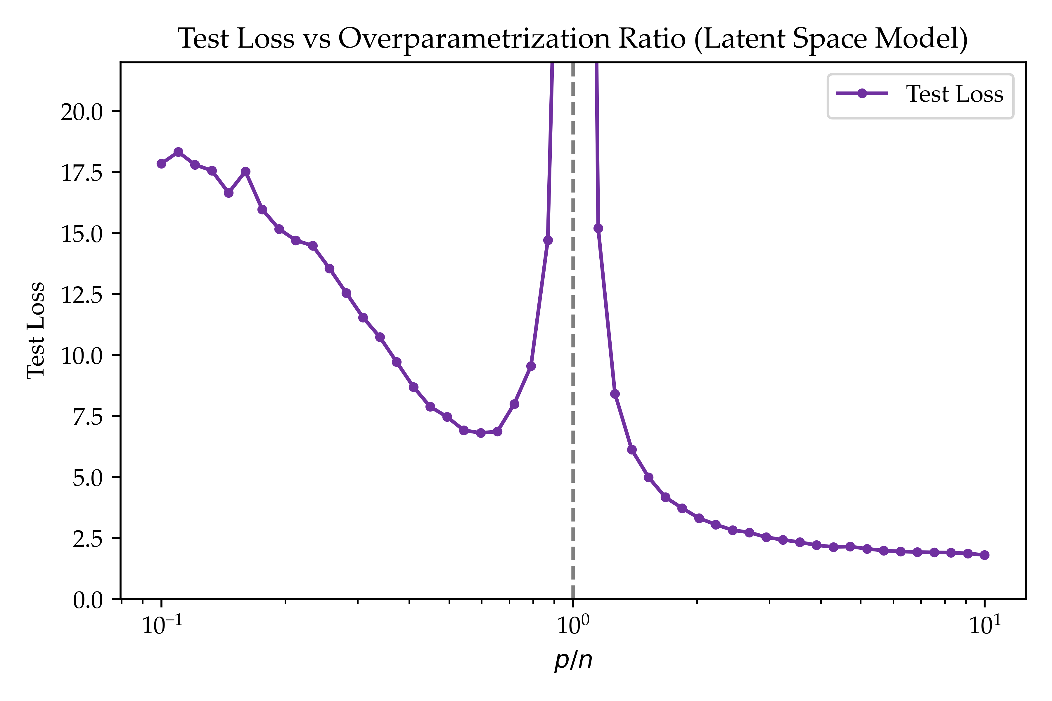
We can now compute the error of models for different parameter counts (like the previous section, we omit the general theorems/proofs). In Figure 3, we plot the error as a function of $p/n$ for a fixed (large) $n$ for $\sigma_{\xi} = 1$ and Gaussian $\theta, W$. As before, we see that the training error decreasing past the transition point $p/n = 1$. Interestingly, the lowest test loss is achieved by sending $p \to \infty$ for a fixed $n$! This shows that overparameterization is optimal for this latent space regression, not just for neural networks.

Summary

It seems that gradient descent magically finds generalizing solutions in the space of interpolating models. This shows that the classical bias-variance trade-off is a flawed picture of model performance. Moreover, all it takes is linear regression to observe this phenomenon. I hope this post was helpful in building intuition, and I highly recommend reading some of the original papers in this space to understand the full picture. Thank you for reading, and feel free to reach out with any questions or thoughts!

Code

The code for this post is available here.