From Entropy to Epiplexity (Interestingness Part 2)

$ \def\R{\mathbb{R}} \def\model{q_\theta} \newcommand{\fd}[2]{D_f(#1 \; \| \; #2)} \newcommand{\Eof}[2]{\mathbb{E}_{#1}\left[#2\right]} \newcommand{\p}[1]{\left(#1\right)} \newcommand{\b}[1]{\left[#1\right]} \newcommand{\br}[1]{\left\{#1\right\}} \newcommand{\KL}[2]{D_{\text{KL}}\p{#1\;||\;#2}} \newcommand{\CE}[2]{\text{H}\p{#1, #2}} \newcommand{\H}[1]{\text{H}\p{#1}} \newcommand{\kde}[1]{\hat{p}_n(#1)} \newcommand{\MSE}{\text{MSE}} $

1/29/2025

Unless you are a whiz at algorithmic information theory, you will find it helpful to read Interestingness Part 1 first.

In the previous post, we discussed classical notions of quantifying information content via information theory and algorithmic complexity. We found that entropy was close to the Kolmogorov complexity at the sample level, whereas Kolmogorov complexity of the distribution captures something else. For example, the uniform distribution is high entropy and high Kolmogorov per sample (suggesting high random information) and low Kolmogorov for the distribution (suggesting low structural information). However, these classical notions would assign low random information to pseudo-random number generators and low structure to the distribution of math proofs (discussed more in depth later).

In this post, we cover how epiplexity (Finzi et al, 2026) correctly resolves these paradoxes via computational constraints. Moreover, we will cover the interesting implications for whether machine learning algorithms extract structure from data.

Failures of complexity and entropy

We first go over two examples that motivate the failures of distributional complexity and entropy. This is a rearrangement of the three paradoxes from the original paper.

Mathematics (clasically low structure, intuitively high structure). A distribution we might believe has high structure is the distribution over all math theorems that type check in Lean in a finite amount of time. However, the Kolmogorov complexity of this distribution is quite low: we can simply write a program that enumerates all finite strings and checks compilation in Lean. More generally, we find it hard to construct examples of distributions that have high $K(P)$.

Pseudo-random number generators (classically low randomness, intuitively high randomness). The data processing inequality says that deterministic functions can not increase the total information content present in data. On the contrary, PRNGs leverage an NP-hard problem to deterministically expand $k$ advice bits (i.e. seed) into $n = \text{poly}(k)$ bits that appear random to any polynomial time algorithm. By the data processing inequality, the entropy of the data can not increase under deterministic functions and is therefore bounded by the entropy of the advice ($\leq k$). On the other hand, to any polynomial time algorithm, the bits would appear random and intuitively contains an entropy closer to $n$ bits.

Between both examples, a common theme is that the intuition deviates from the theory due to time constraints. Epiplexity addresses this by thinking about learning under compute constraints. We first introduce learning.

Learning via minimum description length

So far, our notions of random information (entropy) and structural information (minimum program length for the distribution) have been kept separate from each other. However, when selecting models according to data (i.e. learning), we are interested in balancing both. This classical idea of Occam's razor (selecting the simplest hypothesis that explains the data) can be formalized as minimizing the total description length of describing a hypothesis and describing the data under this hypothesis. More formally, for candidate programs $\mathcal{H}$, the minimum description length is

$$L(x) = \min_{h\in\mathcal{H}} |h| - \Eof{x\sim P}{\log P_h(x)}$$

We can decompose the total description length at the minimizer into its structural component $|h|$ and random component $- \Eof{x\sim P}{\log P_h(x)}$ which we will denote $S_{\infty}(P)$ and $H_{\infty}(P)$ (suggestive of future notation).

Epiplexity

The only difference between MDL is that we will constraint the candidate programs to run in time less than $T(n)$ for length $t$ inputs.

$$L_T(X) = \min_{H \in \mathcal{H}_T} |h| - \Eof{x\sim P}{\log P_h(x)}$$

Similar to MDL we will capture the structural information $|h|$ as the epiplexity $S_T(P)$ and the random information $- \Eof{x\sim P}{\log P_h(x)}$ as the time-bounded entropy $H_T(P)$.

This notion resolves both of the failures we provided earlier.

For math, given infinite compute, we have low epiplexity. However, when restricting the compute, there is a tradeoff between using shorter programs and more accurately capturing the distribution. Balancing both desiderata will likely yield longer math programs that amortize the most repeatable structures in math, increasing the epiplexity relative to the infinite compute regime.

For pseudo-random number generators that expand $k$ random bits into $n = \text{poly}(k)$ bits, we know that the Shannon entropy is upper-bounded by $k$. On the other hand, time-bounded entropy for polynomial $T$ can not be significantly lower than $n$ without violating our cryptographic assumptions. Therefore, time-bounded entropy correctly captures that pseudo-random number generators are effectively random.

Epiplexity for machine learning

Estimating program length via prequential coding

One naive way to estimate the program length is count the number of bits necessary to encode the architecture and parameters. However, the authors point out this might significantly overestimate the length of the shortest program since it is known that neural network weights are highly compressible.

One classical scheme to encode the model is via prequential coding. In this scheme, we only encode the program necessary to initialize the model and encode the data points with respect to the model over the course of training. More specifically,

Initialize the model architecture, weights, and optimizer using a constant number of bits.
At training step $i$, maintain model checkpoint $Q_i$. To compress data point $x_i$, use the prefix code induced by $Q_i$ to entropy code the data point in $-\log Q_i(x_i)$ bits.

The data contained above can be executed as a program to produce the final model: initialize the model, decode the original sample with respect to the current checkpoint, take a gradient update, and repeat for all the data points. However, this coding scheme includes the bits for compressing both the model and the entire dataset. As a post-hoc correction, one can approximate the bits of the $M$ images via entropy coding with the final model checkpoint $Q_M$. Therefore, we can approximate the model description length as

$$\sum_{i\in[M]} -\log Q_i(x_i) + \log Q_M(x_i)$$

or, the area under the loss curve until the terminating loss as visualized as the blue region in Figure 1.

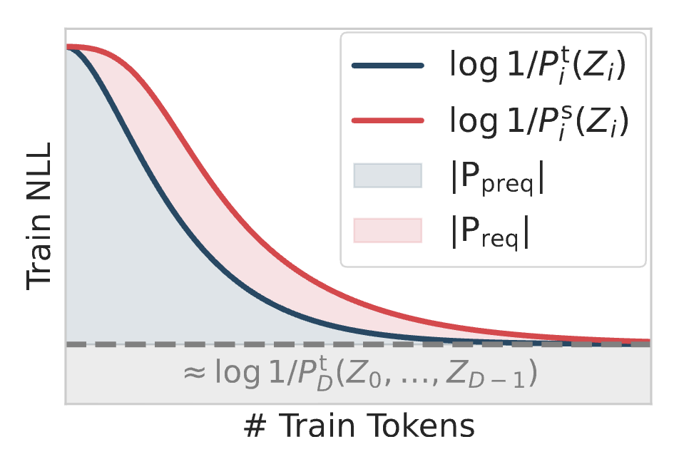
Figure 1: Visualization of prequential coding.

The paper notes that the above coding scheme has a lot of heuristics and alternatively considers requential coding (red region, employing a plausibly better set of heuristics). Fortunately, the authors find that the two metrics correlate empirically, even if requential coding is $2-10\times$ shorter description lengths. Nonetheless, all their main experiments only use prequential coding.

One experiment

The paper has a couple of interesting experiments demonstrating possible applications for epiplexity in the context of data selection. A couple that are worth reading about are the cellular automata as well as what scaling laws imply about epiplexity as a function of compute and modality.

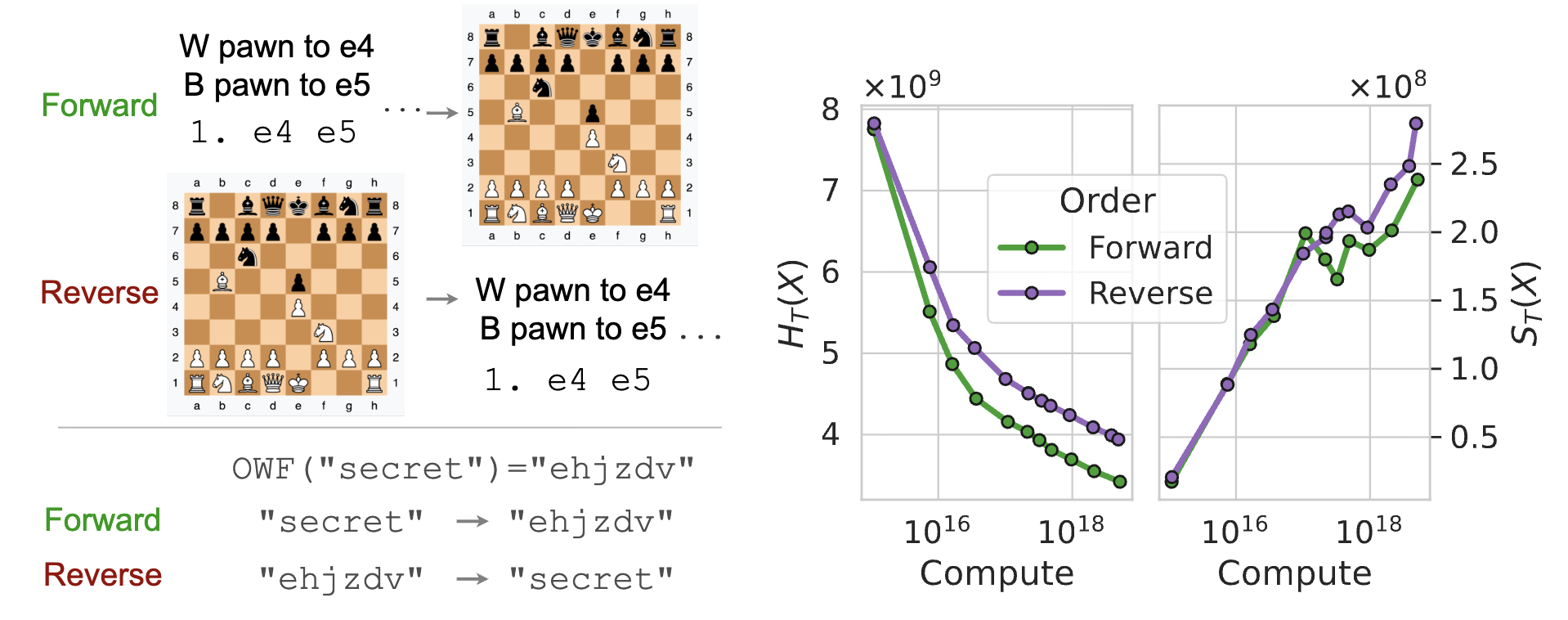
We will cover what I think is the most interesting experiment for the paper surrounding chess. Consider two distinct formats for chess pre-training, as visualized in Figure 2 left: seeing the moves of a game followed by the final chess board (forward), or seeing the final chess board followed by the initial moves (reverse). Both directions have the same loss minimizer since the factorization of the probability distribution (i.e. the order of the tokens) doesn't change the underlying distribution. However, predicting the board given the moves is more computationally easy relative to inferring the moves given the board by marginalizing over all possible games. This is related to a fact that the epiplexity of $f^-1$ is not necessarily close to the epiplexity of $f$ (on the other hand, Kolmogorov complexity barely changes thanks to Levin search).

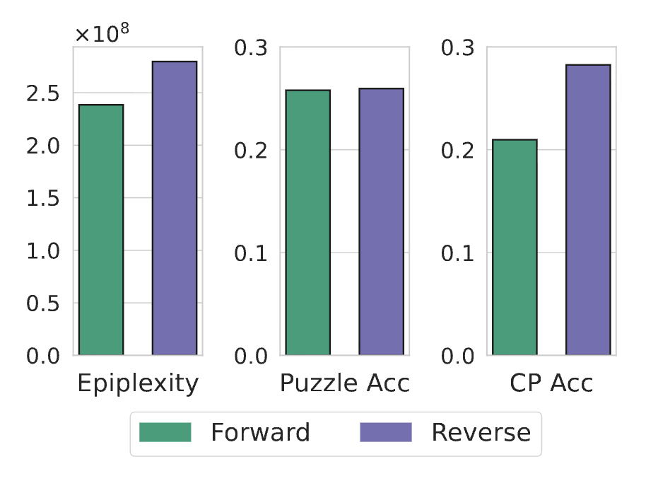
When training on this task, the total loss is higher for the reverse representation, as expected. However, when decomposing into epiplexity and time-bounded entropy, one finds that the epiplexity is higher for reverse training (Figure 2, middle). Intuitively, this captures that the model trained on reverse chess boards has extracted more structure from the task as its more computationally difficult. When testing on OOD chess tasks, the reverse model performs better than the forward model, suggesting that the reverse network generalizes better (Figure 2, right).

Figure 2: Chess example where epiplexity predicts OOD generalization on CP task.

Conclusion

Hopefully you found that epiplexity offers a fresh take on generalization as training for the maximum amount of extracted information. Thank you for reading, and feel free to reach out with any questions or thoughts!