Convex Optimization Theory Agrees with Learning Rate Scheduling

\( \def\R{\mathbb{R}} \def\wavg#1{\overline{f(x_{#1:T})}} \)

2/27/2025

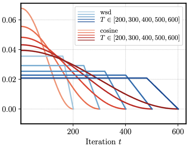
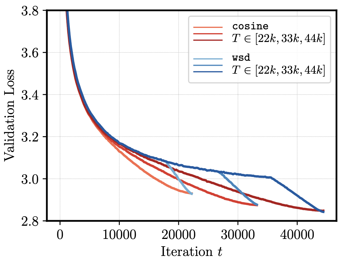
Learning rate schedules nontrivially shape the trajectory of model training as seen in the below figure. The most relevant example is the Warmup-Stable-Decay (WSD) schedule, which keeps a constant learning rate until it linearly decays to zero at the end of training (Figure 1, left). Practitioners have observed that the loss under this schedule (Figure 1, right) decreases slower than a standard cosine schedule until the learning rate decays, at which point the loss sharply decreases (Hu et al, 2024).

Why does this happen? The recent amazing papers Defazio et al, 2024 and Schaipp et al, 2025 shed some light on this question by finding an extremely simple toy model which replicates these empirical phenomena. The theorem maps a sequence of learning rates and expected gradient norms to an upper bound on the loss over the course of training. Their proof relies on a simple trick to extend a classical convex optimization result to the final iterate of a variable learning rate schedule.

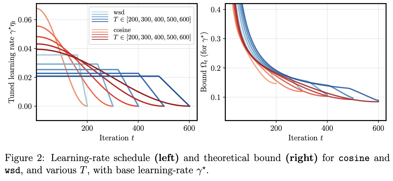
Though the theorem gives a loose upper bound (that gets worse for more non-linear functions), it ends up correctly predicting the "shape" of the loss curve over the course of real training (Figure 2). The predictive nature is incredibly impressive; even though deep learning models and algorithms are incredibly non-convex, this toy model shows that this complexity is not necessary to induce the phenomenon of interest. The original papers contain a simple proof and detailed discussion of empirical results; this post is dedicated to a personally more intuitive version of the proof. I am very impressed at the predictive nature of this toy model and hope you find it interesting as well!

Setup

Suppose we have training samples $s \in \mathcal{S}$ with parameters $x \in \R^d$. We'll consider a loss function $f : \R^D \times \mathcal{S} \to \R$ that computes the loss of the parameters for a single sample. We will overload notation and let $f : \R^d \to \R$ be the expected loss of the parameters, defined as $f(x) = \mathbb{E}_{s \sim \mathcal{P_S}}[f(x, s)]$. We note that the gradient $g_t = \nabla f(x_t, s_t)$ is random over the choice of training sample $s_t$. The learning rate at time $t$ will be given by $\eta_t \in \R^+$. Our training trajectory is then given by the update

\begin{aligned} x_{t+1} &= x_t - \eta_t g_t \end{aligned}

where $x_{t+1}$ is also random over the choice of training sample. We assume that the loss function is convex, which means

\begin{aligned} f(y) - f(x_t) \geq \langle g_t, y - x_t \rangle \end{aligned}

Theorem

Take the optimal parameters $x_*$ and define $D := ||x_1 - x_*||_2$. Then, the theorem bounds how far the loss of the final iterate is from optimal.

\begin{aligned} \mathbb{E}[f(x_T) - f(x_*)] \leq & \frac{1}{2\sum_{t=1}^{T} \eta_t} \left[D^2 + \sum_{t=1}^{T} \eta_t^2 ||g_t||_2^2\right] \\ + & \frac{1}{2} \sum_{k=1}^{T-1} \frac{\eta_k}{\sum_{t=k+1}^{T} \eta_t} \left(\frac{1}{\sum_{t=k}^{T} \eta_t} \sum_{t=k}^{T} \eta_t ||g_t||_2^2\right) \end{aligned}

We will first go over the proof. If you want to skip directly to the application of this proof, you can go here.

Proof

The proof hinges on a key lemma that bounds the average loss of the parameters over time (weighted by the learning rate schedule); the bound only requires the convexity of the loss function. The papers' contribution is to cleverly apply this result to bound the loss of the final iterate.

As a useful intermediate quantity, we will define the weighted average loss of the parameters over time as

\begin{aligned} \wavg{k} := \frac{\sum_{t=k}^{T} \eta_t \mathbb{E}[f(x_t)]}{\sum_{t=k}^{T} \eta_t} \end{aligned}

Bounding average loss of iterates

For reference parameters $u \in \R^d$, we want to bound the average loss of the parameters with respect to $u$, or $\wavg{1} - f(u)$. The following lemma bounds $(\sum_{t\in[T]} \eta_t)(\wavg{1} - f(u))$, which simplifies to $\sum_{t\in[T]} \eta_t \mathbb{E}[f(x_t) - f(u)]$. This bound involves the initial distance from $u$ and the gradient norms of each step.

Lemma 1: For any $u \in \R^d$ and any training trajectory $x_t, \eta_t, g_t$,

\begin{aligned} \sum_{t\in[T]} \eta_t \mathbb{E}[f(x_t) - f(u)] \leq \frac{1}{2} \mathbb{E} ||x_1 - u||_2^2 + \frac{1}{2} \sum_{t=1}^{T} \eta_t^2 \mathbb{E} ||g_t||_2^2 \end{aligned}

Proof: The proof uses the convexity of $f$ to relate the gradient norm of each step to the distance from the reference parameter $u$. The full proof is in Appendix A.1.

Bounding loss of final iterate

How can we use this to bound the loss of the final iterate, given by $\mathbb{E}[f(x_T) - f(x_*)]$? To handle this, we will first introduce the average iterate we saw in the previous lemma.

\begin{aligned} \mathbb{E}\left[f(x_T) - f(x_*)\right] = \mathbb{E}\left[f(x_T) - \wavg{1}\right] + \mathbb{E}\left[\wavg{1} - f(x_*)\right] \end{aligned}

The second term is exactly handled by the previous lemma for $u = x_*$. We now focus on the first term. A priori, it seems difficult to apply our previous lemma because the average iterate is on the wrong side of the subtraction. To handle this, Defazio et al, 2024 cleverly rearranges this term as distances of average iterates from $x_k$ for $k \in [T-1]$. We will prove this in the next lemma.

Lemma 2: For any sequence $x_t, \eta_t$ (not necessarily a training trajectory),

\begin{aligned} f(x_T) - \wavg{1} = \sum_{k=1}^{T-1} \frac{\eta_k}{\sum_{t=k+1}^{T} \eta_t} \left(\wavg{k} - f(x_k)\right) \end{aligned}

Proof: For a brief explanation, each term of the summation is equivalent to $\wavg{k+1} - \wavg{k}$, telescoped to give us $\wavg{T} - \wavg{1} = f(x_T) - \wavg{1}$. The full proof is in Appendix A.2.

After rewriting, we can apply our previous lemma to bound the $k$th term of the sum by setting $u = x_k$ and simulating the training trajectory from $x_k$ to $x_T$. This results in the initial distance being zero, resulting in the trajectory being bounded by the gradient norms of each step. Putting everything together, we get the following bound.

\begin{aligned} \mathbb{E}\left[f(x_T) - f(x_*)\right] = & \mathbb{E}\left[f(x_T) - \wavg{1}\right] + \mathbb{E}\left[\wavg{1} - f(x_*)\right] \\ = & \sum_{k=1}^{T-1} \frac{\eta_k}{\sum_{t=k+1}^{T} \eta_t} \mathbb{E}\left[\wavg{k} - f(x_k)\right] + \mathbb{E}\left[\wavg{1} - f(x_*)\right]\\ \leq & \frac{1}{2} \sum_{k=1}^{T-1} \frac{\eta_k}{\sum_{t=k+1}^{T} \eta_t} \left(\frac{1}{\sum_{t=k}^{T} \eta_t} \sum_{t=k}^{T} \eta_t ||g_t||_2^2\right) \\ + & \frac{1}{2\sum_{t=1}^{T} \eta_t} \left[D^2 + \sum_{t=1}^{T} \eta_t^2 ||g_t||_2^2\right] \end{aligned}

This completes the proof :))

Application

Due to empirical observation, the paper assumes that the gradient norm is constant over time ($\mathbb{E}||g_t||^2_2 = G$), more on this later. With this assumption, we can derive a closed form expression for the loss of the final iterate. As discussed in the introduction, the shape of the bound closely matches empirical loss curves for WSD and cosine schedules. The paper also discusses many settings where this theorem correctly prescribes an action to take in practice. We'll work through the simplest one: tuning the learning rate for a fixed schedule.

We will rewrite the learning rate $\eta_t$ as $\gamma * \mu_t$ where $\gamma$ is the maximum learning rate and $\mu_t \in [0, 1]$ is a normalized learning rate schedule. Then, the theorem (with slight rearrangement) becomes

\begin{aligned} \mathbb{E}[f(x_T) - f(x_*)] \leq & \frac{1}{\gamma}\left[\frac{D^2}{2 \sum_{t=1}^{T} \mu_t}\right] \\ + & \gamma \left[\frac{1}{2\sum_{t=1}^{T} \mu_t} \sum_{t=1}^{T} \mu_t^2 G\right. \\ & + \left.\frac{1}{2} \sum_{k=1}^{T-1} \frac{\mu_k}{\sum_{t=k+1}^{T} \mu_t} \left(\frac{1}{\sum_{t=k}^{T} \mu_t} \sum_{t=k}^{T} \mu_t G\right)\right] \end{aligned}

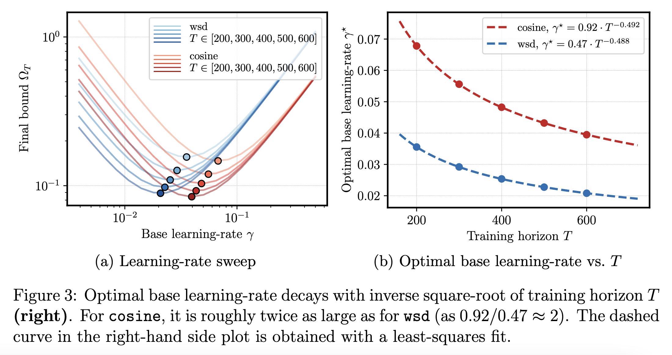
Under this parameterization, we can rewrite the bound as $\frac{\mathcal{T}_1}{\gamma} + \mathcal{T}_2\gamma$ for expressions $\mathcal{T}_1, \mathcal{T}_2$ that only depend on the learning rate schedule. Therefore, for a given schedule, the bound prescribes using learning rate $\gamma = \sqrt{\frac{\mathcal{T}_1}{\mathcal{T}_2}}$. Obviously, this will be off by important constants. However, it does predict the scaling behavior of optimal learning rates. For example, the bound (numerically) predicts that for a fixed schedule, the optimal learning rate is roughly proportional to $\frac{1}{\sqrt{T}}$ (Figure 3). This is exactly what people observe in practice (Shen et al, 2024)! The paper has more examples, such as showing the optimal cooldown duration for WSD is the entire training duration and that you can transition between learning rates smoother.

Gradient norm assumption

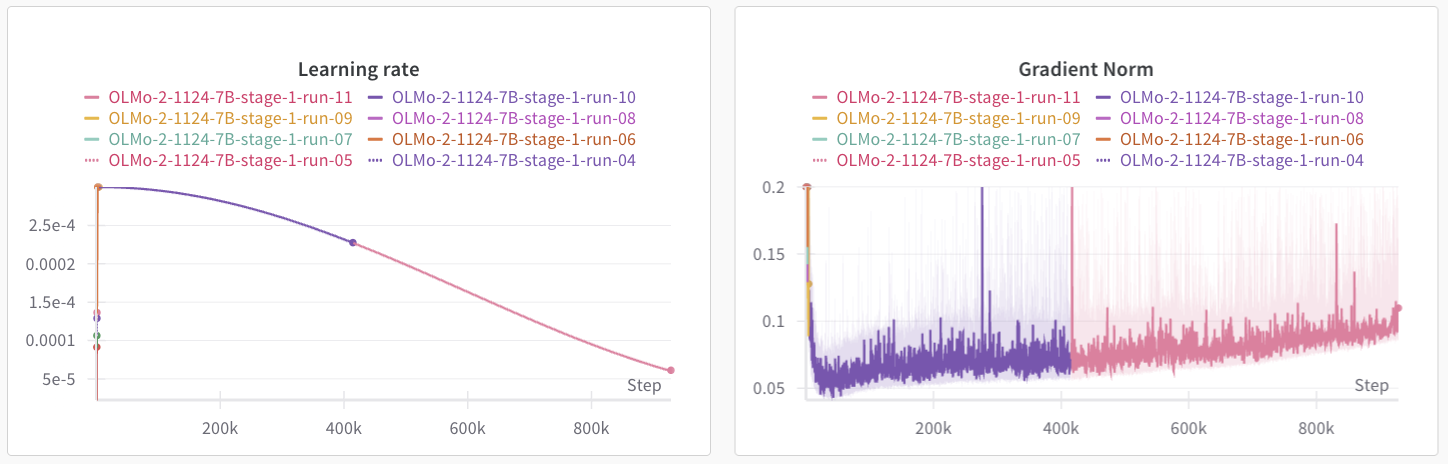
The paper assumes that the gradient norm is constant over time ($\mathbb{E}||g_t||^2_2 = G$) which does not seem to be the case for training. For example, you can look at the gradient norm over the course of training for OLMo 2 7B (OLMo et al, 2025) in Figure 4. The gradient norm sharply decreases during the start of training before slowly increasing for the rest of training. My understanding is that the optimal schedule for this gradient norm involves a quick warmup at the start of training, which aligns well with common practices. Defazio et al, 2024 has a more nuanced treatment.

Conclusion

This toy model is extremely simple yet predictive of how learning rate schedules shape the training trajectory. In some preliminary experiments, I found that the bound makes some accurate predictions regarding the optimal data ordering where data points differ in their expected gradient norms, but that's for another post. Please refer to the original papers for more details, extensions, and empirical results. Thank you for reading, and feel free to reach out with any questions or thoughts!

Appendix

A.1: Proof of Lemma 1

Lemma 1: For any $u \in \R^d$ and any training trajectory $x_t, \eta_t, g_t$,

\begin{aligned} \sum_{t\in[T]} \eta_t \mathbb{E}[f(x_t) - f(u)] \leq \frac{1}{2} \mathbb{E} ||x_1 - u||_2^2 + \frac{1}{2} \sum_{t=1}^{T} \eta_t^2 \mathbb{E} ||g_t||_2^2 \end{aligned}

Proof: We relate the gradient norm of each step to the distance from reference parameter $u$.

\begin{aligned} \mathbb{E}||x_{t+1} - u||_2^2 &= \mathbb{E}||x_t - \eta_t g_t - u||_2^2 \\ &= \mathbb{E}[||x_t - u||_2^2 - 2\eta_t \langle g_t, x_t - u \rangle + \eta_t^2 ||g_t||_2^2] \\ &\leq \mathbb{E}[||x_t - u||_2^2 - 2\eta_t (f(x_t, s_t) - f(u, s_t)) + \eta_t^2 ||g_t||_2^2] && \text{[convexity]} \end{aligned}

The last inequality uses convexity of $f$. By taking the expectation and rearranging terms, we get

\begin{aligned} 2\eta_t \mathbb{E}[f(x_t) - f(u)] &\leq \mathbb{E}[||x_t - u||_2^2] - \mathbb{E}[||x_{t+1} - u||_2^2] + \eta_t^2 \mathbb{E}[||g_t||_2^2] \end{aligned}

Summing over $t \in [T]$ gives a telescoping series for the distances:

\begin{aligned} 2\sum_{t=1}^T \eta_t \mathbb{E}[f(x_t) - f(u)] &\leq \mathbb{E}[||x_1 - u||_2^2] - \mathbb{E}[||x_{T+1} - u||_2^2] + \sum_{t=1}^T \eta_t^2 \mathbb{E}[||g_t||_2^2] \\ &\leq \mathbb{E}[||x_1 - u||_2^2] + \sum_{t=1}^T \eta_t^2 \mathbb{E}[||g_t||_2^2] \end{aligned}

Dividing both sides by 2 gives the desired result.

A.2: Proof of Lemma 2

Lemma 2: For any sequence $x_t, \eta_t$ (not necessarily a training trajectory),

\begin{aligned} f(x_T) - \wavg{1} = \sum_{k=1}^{T-1} \frac{\eta_k}{\sum_{t=k+1}^{T} \eta_t} \left(\wavg{k} - f(x_k)\right) \end{aligned}

Proof: Our goal with this lemma is to rewrite $f(x_T) - \wavg{1}$ as a sum of terms of the form $\wavg{k} - f(x_k)$. To shed some light on this term, we note that each term of the summation is actually $\wavg{k+1} - \wavg{k}$, telescoped to give us $\wavg{T} - \wavg{1} = f(x_T) - \wavg{1}$. In the lemma statement, the $k$th term of the summation is peeling off $x_k$ from $\wavg{1}$ by matching it to an appropriate weighted average. This continues until we have peeled off all the $x_k$ from $\wavg{1}$.

As for a rigorous proof, it suffices to show that the $k$th term of the summation is $\wavg{k+1} - \wavg{k}$. We directly compute this term:

\begin{aligned} \wavg{k+1} - \wavg{k} &= \frac{\sum_{t=k+1}^{T} \eta_t f(x_t)}{\sum_{t=k+1}^{T} \eta_t} - \frac{\sum_{t=k}^{T} \eta_t f(x_t)}{\sum_{t=k}^{T} \eta_t} \\ &= \frac{\sum_{t=k+1}^{T} \eta_t f(x_t)}{\sum_{t=k+1}^{T} \eta_t} - \frac{\eta_k f(x_k) + \sum_{t=k+1}^{T} \eta_t f(x_t)}{\eta_k + \sum_{t=k+1}^{T} \eta_t} \\ &= \frac{(\sum_{t=k+1}^{T} \eta_t f(x_t))(\eta_k + \sum_{t=k+1}^{T} \eta_t) - (\eta_k f(x_k) + \sum_{t=k+1}^{T} \eta_t f(x_t))(\sum_{t=k+1}^{T} \eta_t)}{(\sum_{t=k+1}^{T} \eta_t)(\eta_k + \sum_{t=k+1}^{T} \eta_t)} \\ &= \frac{\eta_k\sum_{t=k+1}^{T} \eta_t f(x_t) - \eta_k f(x_k)\sum_{t=k+1}^{T} \eta_t}{(\sum_{t=k+1}^{T} \eta_t)(\eta_k + \sum_{t=k+1}^{T} \eta_t)} \\ &= \frac{\eta_k\sum_{t=k}^{T} \eta_t f(x_t) - \eta_k f(x_k)\sum_{t=k}^{T} \eta_t}{(\sum_{t=k+1}^{T} \eta_t)(\sum_{t=k}^{T} \eta_t)} \\ &= \frac{\eta_k}{\sum_{t=k+1}^{T} \eta_t} \left(\frac{\sum_{t=k}^{T} \eta_t f(x_t)}{\sum_{t=k}^{T} \eta_t} - f(x_k)\right) \\ &= \frac{\eta_k}{\sum_{t=k+1}^{T} \eta_t} \left(\wavg{k} - f(x_k)\right) \end{aligned}

Therefore, summing over $k \in [T-1]$ gives us a telescoping series:

\begin{aligned} \sum_{k=1}^{T-1} \frac{\eta_k}{\sum_{t=k+1}^{T} \eta_t} \left(\wavg{k} - f(x_k)\right) &= \sum_{k=1}^{T-1} (\wavg{k+1} - \wavg{k}) \\ &= \wavg{T} - \wavg{1} \\ &= f(x_T) - \wavg{1} \end{aligned}

And we're done!