Probabilistic Inference in Language Models via Twisted Sequential Monte Carlo
\( \def\R{\mathbb{R}} \def\wavg#1{\overline{f(x_{#1:T})}} \newcommand{\clip}[3]{\left[#1\right]^{#3}_{#2}} \def\sT{s_{1:T}} \def\st{s_{1:t}} \def\st1{s_{1:t}} \def\partition{\mathcal{Z}} \def\base{p_0} \def\potential{\phi} \def\target{\sigma} \def\targetRL{\sigma_{\text{RL}}} \def\itarget{\pi} \def\twist{\psi} \newcommand{\unnorm}[1]{\tilde{#1}} \newcommand{\p}[1]{\left(#1\right)} \newcommand{\b}[1]{\left[#1\right]} \newcommand{\br}[1]{\left\{#1\right\}} \newcommand{\KL}[1]{D_{\text{KL}}\p{#1}} \newcommand{\Eof}[2]{\mathbb{E}_{#1}\left[#2\right]} \)7/25/2025
Probabilistic Inference in Language Models via Twisted Sequential Monte Carlo (Zhao et al, 2024) describes cool connections between the probabilistic inference approach and reinforcement learning approach to sampling from a potential/reward function. This post is mostly notes to simplify the detailed exposition of the paper. We closely follow the SMC exposition and restructure the connection to RL. Thanks to many discussions with Konwoo and my reading group friends Arthur, Peter, and Gabe.
Problem statement
You are interested in decoding $T$ tokens $\sT$ from a base language model denoted $\base$. You have a potential function denoted $\potential(\sT)$ that can tell you how desirable a response is. For example, is $\sT$ a valid math proof, is $\sT$ not toxic, etc. This potential can only be evaluated on full sequences.
You are given an auto-regressive base model $\base$ and you are interested in sampling from this distribution reweighted by the potential function. Specifically, you want to sample from target density $\target(\sT)$ defined as
\begin{aligned} \sigma(\sT) &:= \frac{1}{\partition_\sigma} \base(\sT) \potential(\sT) \\ \text{for } \unnorm{\target}(\sT) &:= \base(\sT)\potential(\sT) \\ \text{and } \partition_\sigma &:= \sum_{\sT} \unnorm{\target}(\sT) \end{aligned}
where $\unnorm{\target}(\sT)$ corresponds to the un-normalized target density and $\partition_\sigma$ is the partition function, or constant that makes this a probability distribution.
Summary of approaches
How can we sample from the target distribution? One approach is to perform reinforcement learning to directly learn the correct policy: specifically, if you perform RL with KL regularization $\beta$ and reward function $r(\sT) = \exp\p{\frac{\phi(\sT)}{\beta}}$, the loss minimizer (i.e. constrained reward maximizer) corresponds exactly to $\target(\sT)$ (which we'll prove later).
A second approach comes from sampling and probabilistic inference. Instead of changing the base policy, one can sample responses and reweight them by the potential function. Though this would eventually produce samples from the true distribution with infinite samples, it is plagued with variance for finite samples since the base policy is imperfect. This paper uses Sequential Monte Carlo, which reduces the variance by constructing a sequence of intermediate distributions that terminates in the target distribution alongside a clever proposal distribution. The paper aims to learn twist functions that best approximate both the desired intermediate distributions and the optimal proposal distribution
We will first cover the SMC-style twist function approaches, discuss its correspondence with RL, and show how to compare approaches by their ability to estimate the partition function. We will omit the conditioning application as it felt less central to my interests.
Motivating/using SMC and Twists
Naive importance sampling
Ok, let's first try to go down this sampling route. Note that we can readily evaluate the un-normalized density $\unnorm{\target}$. Given an arbitrary proposal distribution $q$, we can use this sample from $\target$ using self-normalized importance sampling (SNIS). First, define importance sampling weights $w(\sT)$ as $w(\sT) := \frac{\unnorm{\target}(\sT)}{q(\sT)}$. Now, given multiple responses $\sT^i$ for $i$ indexed in $[K]$, we can approximate sampling from $\target$ by sampling an index $\omega$ from the categorical distribution $\text{cat}\p{\left\{\frac{w(\sT^i)}{\sum_{j\in[K]}w(\sT^j)}\right\}_{i\in[K]}}$. Note that since we are sampling with replacement and some samples have higher weight, it is likely that some of the proposed samples are duplicated.
In the infinite sample limit $K \to \infty$, this produces true samples from the target $\target$. Unfortunately, for finite samples, its success is defined by how close the proposal $q$ is to the target $\target$. For example, if the proposal was equal to the target $q(\sT) = \sigma(\sT)$, then every importance weight would be $\partition_\sigma$ and the variance of the importance weights would be $0$, corresponding to good finite sample SNIS.
Sequential Monte Carlo (SMC)
We want a lower variance proposal distribution so that we get a better sampler. The focus of SMC is to construct a proposal distribution that's closer to the target distribution. This is done by constructing a sequence of intermediate target distributions $\br{\itarget_t(\st)}_{t\in[T]}$. For example, diffusion can be viewed as SMC by setting the intermediate targets to be Gaussian corruptions of the target data distribution. For our discussion, each intermediate distribution will be over length $t$ prefixes. SMC starts with $K$ empty sequences and partially updates them in steps $1, \ldots, t, \ldots, T-1$ in the following manner
- Propose: sample one new token from the proposal $q(s^k_t | s^k_{1:t-1})$ for each sequence $k$
- Weight: assuming we have access to the likelihoods of the intermediate distributions $\itarget_t$, assign a weight to each sample $s^k_{1:t}$ as if it was from ${\itarget}_t$ via weighting function $w_t(\st) := \frac{\unnorm{\itarget}_t(\st)}{\unnorm{\itarget}_{t-1}(s_{1:t-1})q(s_t | s_{1:t-1})}$
- Resample: use self-normalized importance sampling to samples from $K$ sequences with weights $\frac{w(\st^i)}{\sum_{j\in[k]}w(\st^j)}$. These samples are now effectively drawn from $\itarget_t(\st)$.
To ensure that our final samples are from our target distribution of interest in this formulation, we simply set $\pi_T = \sigma_T$. Now, it doesn't matter whether are sampling the intermediate distributions since this final resampling step corrects for any proposal, similar to naive importance sampling.
Twisted Sequential Monte Carlo
The key design decision of twisted SMC methods is to define the intermediate target distributions as the true marginals. In other words, the desired targets $\pi_t(\st)$ are equivalent to $\target(\st)$ for all $t$. To achieve this, we will construct twist functions $\twist_t(\st)$ that signify the difference between our base policy and the desired intermediate distributions. Namely,
\begin{aligned} \itarget_t(\st) = \begin{cases} \frac{1}{\partition^\twist_t} \base(\st) \twist_t(\st) & t\neq T\\ \frac{1}{\partition^\potential} \base(\st) \potential_t(\st) & t=T \\ \end{cases} \end{aligned}
Now, we can simply plug in these definitions for the intermediate distributions and (ignoring constants) derive the importance sampling weights of
\begin{equation}\label{smc-weight} \begin{split} w_t(\st) &= \frac{\unnorm{\itarget}_t(\st)}{\unnorm{\itarget}_{t-1}(s_{1:t-1})q(s_t | s_{1:t-1})} \\ &\propto \frac{\base(\st)\twist_{t}(s_{1:t})}{q(s_t | s_{1:t-1})\base(s_{1:t-1})\twist_{t-1}(s_{1:t-1})} \\ &= \frac{\base(s_t | s_{1:t-1})\twist_{t}(s_{1:t})}{q(s_t | s_{1:t-1})\twist_{t-1}(s_{1:t-1})} \label{eq:smc-weight} \\ \end{split} \end{equation}
Note that we if we have horrendous twist functions for steps $[T-1]$, we might not actually be sampling from our intermdiate target distribution of interest $\itarget$. However, this is totally fine since the final twist function $\twist_T$ is always correct and will derive unbiased estimates of the correct importance weights.
Optimal twists
The correct twists correspond to sampling from the true marginal and would result in $\itarget_t(\st) = \target(\st)$. This is equivalent to reweighing each prefix by its future return according to the base policy, or
\begin{equation}\label{eq:twist-marginal}\twist_t^*(\st) \propto \sum_{s_{t+1:T}} \base(s_{t+1:T}|\st)\potential(\sT)\end{equation}
This can be further decomposed into a step-wise consistency condition which RL people might find similar to the Bellman equation (more later)
\begin{equation}\label{eq:twist-bellman}\twist_t^*(\st) \propto \sum_{s_{t+1}} \base(s_{t+1} | \st)\twist_t^*(s_{1:t+1})\end{equation}
Choice of proposal distribution
We can utilize any proposal distribution $q$. The most straightforward choice is using the base policy $q = \base$. However, this isn't going to be the lowest variance proposal. Since the variance minimizing proposal choice $q_t^\pi$ would result in the weights $w_t$ shown in (1) to be constant, it is given by
\begin{aligned} q_t^\pi(s_t | s_{1:t-1}) &\propto \frac{\itarget_t(\st)}{\itarget_{t-1}(s_{1:t-1})} \\ &= \frac{\frac{1}{\partition^\twist_t}\base(\st)\twist_t(\st)}{\frac{1}{\partition_{t-1}^\twist} \base(s_{1:t-1})\twist_{t-1}(s_{1:t-1})} \\ &\propto \base(s_t | s_{1:t-1})\twist_t(\st) && \text{[$\twist_{t-1}(s_{t-1})$ is constant wrt $s_t$]}\\ &= \frac{1}{\partition^\pi_t(s_{1:t-1})}\base(s_t | s_{1:t-1})\twist_t(\st)\\ \end{aligned}
for a new normalizing constant $\partition^\pi_t(s_{1:t-1}) = \sum_{s_t} \base(s_t | s_{1:t-1})\twist_t(\st)$. When the twist function $\twist_t$ is parameterized as an auto-regressive transformer that outputs a number per next token choice, we can compute $\partition^\pi_t(s_{1:t-1})$ as the inner product of two vectors from two forward passes. Since the $\potential(\sT)$ likely does not share this property of being able to output a vector conditioned on $T-1$ tokens, we first learn an approximation $\twist_T$ that outputs a vector. We resample according to this and then further importance sample using $\frac{\potential(\sT)}{\twist_T(\sT)}$. I found it kind of funny that the twist function was being used both for the SMC resampling and for the proposal sampling.
Learning twists
So far, we have shown how to use given twist functions: for each intermediate target distribution, utilize your (twisted) proposal and resample according to the twist functions before reweighting by the true potential for an unbiased estimate. Now, we are interested in learning the desired twist functions to use for the proposal + resampling steps.
We now parameterize our twist functions with parameters $\theta$ as $\twist_t^\theta(\st)$, which implicitly define $\itarget_t^\theta(\st)$ as earlier. We are interested in having our intermediate targets line up with the true marginal targets $\sigma(\st)$.
Contrastive Twist Learning
Suppose we are interested in distribution-matching without mode collapsing, which corresponds to minimizing forward KL divergence instead of reverse KL divergence (distinction sharpened in RL section). The contrastive twist learning (CTL) loss sets this up token-wise as
$$\mathcal{L}_{\text{CTL}}(\theta) := \sum_{t\in[T]} \KL{\sigma(\st) || \itarget_t^\theta(\st)}$$
We can work through the gradient of this objective using the definition of $\itarget_t^\theta$.
\begin{aligned} & -\nabla_\theta \mathcal{L}_{\text{CTL}}(\theta) \\ &= -\sum_{t\in[T]} \Eof{\st \sim \target(\st)}{\nabla_\theta \p{\log \target(\st) - \log \itarget_t^{\theta}(\st)}} \\ &= \sum_{t\in[T]} \Eof{\st \sim \target(\st)}{\nabla_\theta \log \itarget_t^{\theta}(\st)} \\ &= \sum_{t\in[T]} \Eof{\st \sim \target(\st)}{\nabla_\theta \p{\log \base(\st) + \log \twist^\theta_t(\st) - \log \sum_{\st'} \base(\st')\twist^{\theta}_t(\st')}} \\ &= \sum_{t\in[T]} \Eof{\st \sim \target(\st)}{\nabla_\theta \log \twist^\theta_t(\st)} - \nabla_\theta \log \sum_{\st'} \base(\st')\twist^{\theta}_t(\st') \\ &= \sum_{t\in[T]} \Eof{\st \sim \target(\st)}{\nabla_\theta \log \twist^\theta_t(\st)} - \frac{\nabla_\theta \sum_{\st} \base(\st)\twist^{\theta}_t(\st)}{\sum_{\st'} \base(\st')\twist^{\theta}_t(\st')} && \text{[$\nabla_\theta \log f(x) = \nabla f(x)/f(x)$]} \\ &= \sum_{t\in[T]} \Eof{\st \sim \target(\st)}{\nabla_\theta \log \twist^\theta_t(\st)} - \frac{\sum_{\st} \base(\st)\twist^{\theta}_t(\st)\nabla_\theta\log \twist^{\theta}_t(\st)}{\sum_{\st'} \base(\st')\twist^{\theta}_t(\st')} && \text{[$\nabla_\theta f(x) = f(x)\nabla\theta \log f(x)$]}\\ &= \sum_{t\in[T]} \Eof{\st \sim \target(\st)}{\nabla_\theta \log \twist^\theta_t(\st)} - \sum_{\st}\frac{\base(\st)\twist^{\theta}_t(\st)}{\sum_{\st'} \base(\st')\twist^{\theta}_t(\st')}\nabla_\theta\log \twist^{\theta}_t(\st) \\ &= \boxed{\sum_{t\in[T]} \Eof{\st \sim \target(\st)}{\nabla_\theta \log \twist^\theta_t(\st)} - \Eof{\st \sim \itarget_t^\theta(\st)}{\nabla_\theta \log \twist^{\theta}_t(\st)}} \\ \end{aligned}
Now that we've derived the gradient, we notice it has a nice interpretation. Specifically, it contrasts samples taken from the true marginal $\target(\st)$ and the parameterized intermediate target $\itarget_t^\theta$, encouraging samples to look more like the true marginal instead of the parameterized targets. Therefore, it requires a source of positive samples for the right term and negative samples for the left term. Since we can not do this exactly, we will estimate these expectations.
- Negative samples: We can estimate the sampling distribution for the negatives by sampling from $\itarget_t$ as we described earlier. We are allowed to choose which proposal we want since both will result in samples from $\itarget_t$.
- Positive samples: If we had access to ground truth samples, we can plug them in here. If we don't have access to these, then we can use our sampling algorithms to approximate them. Specifically, to generate positive samples $\st$, we can use the full twisted SMC algorithm to generate approximate samples $sT$ and trunctate them to length $t$. At first glance, this might appear to be the same as the negative samples. However, these prefixes are reweighted based on the potential of the full sequences, whereas the negative samples only use the likely inaccurate twists up to $t$.
Nice! Are there other ways to learn twist functions? (the below descriptions are not incredibly detailed)
- Noise Contrastive Estimation: Twist functions can also be seen as energy models, where the goal is to learn $E(\st) := \log \sigma(\st) - \log \base(\st)$. In the EBM literature, this is trained via noise contrastive estimation by performing binary classification between real samples and base samples. This similarly requires sampling under both the true marginal distribution and the twisted approximation of the distribution, leveraging similar machinery to the CTL loss.
- Soft RL: We can use value-based RL to guide our training of twist functions. We discuss the basic idea of this approach later. Briefly, this method often enforces the consistency loss described in Equation \eqref{eq:twist-bellman}
- FUDGE: Briefly, we can enforce the full consistency loss as described in Equation \eqref{eq:twist-marginal}.
Connection to RL: Directly learning policies
In RL, the goal is to directly learn a policy with the desired properties instead of learning twist functions. Standard RL is policy learning with reverse KL, and distributional RL is policy learning with forward KL.
Standard RL
First let's set up RL independent of all this. You are given reward function $r(\sT)$ and base policy $\base(\sT)$. For simplicity and connection to LLMs (which are contextual bandits), we will assume that this reward is only assigned to full sequences and is zero otherwise. RL can be KL-constrained, which it means that it balances maximizing reward with remaining close to the original policy with regularization strength $\beta$ (I think they flipped $\beta$ here so low $\beta$ means high regularization). Overloading notation, the goal is to find a policy $q^{\theta}(\sT)$ that maximizes the reward
\begin{aligned} & \Eof{\sT \sim q^{\theta}}{r(\sT)} - \frac{1}{\beta}\KL{q^{\theta}(\sT) || \base(\sT)} \\ &= \Eof{\sT \sim q^{\theta}}{r(\sT)} - \Eof{\sT \sim q^{\theta}}{\frac{1}{\beta}(\log q^{\theta}(\sT) - \log \base(\sT))} \\ &= -\frac{1}{\beta} \left(\Eof{\sT \sim q^{\theta}}{\log q^{\theta}(\sT) - \beta r(\sT) - \log \base(\sT)}\right) \\ &= -\frac{1}{\beta} \left(\Eof{\sT \sim q^{\theta}}{\log q^{\theta}(\sT) - \beta r(\sT) - \log \base(\sT) + \partition_{\targetRL}} - \partition_{\targetRL}\right)\\ &= -\frac{1}{\beta} \KL{q^{\theta}(\sT) || \targetRL(\sT)} - \frac{1}{\beta}\partition_{\targetRL}\\ \text{for }\targetRL(\sT) &:= \frac{1}{\partition_{\targetRL}} \base(\sT) e^{\beta r(\sT)} \end{aligned}
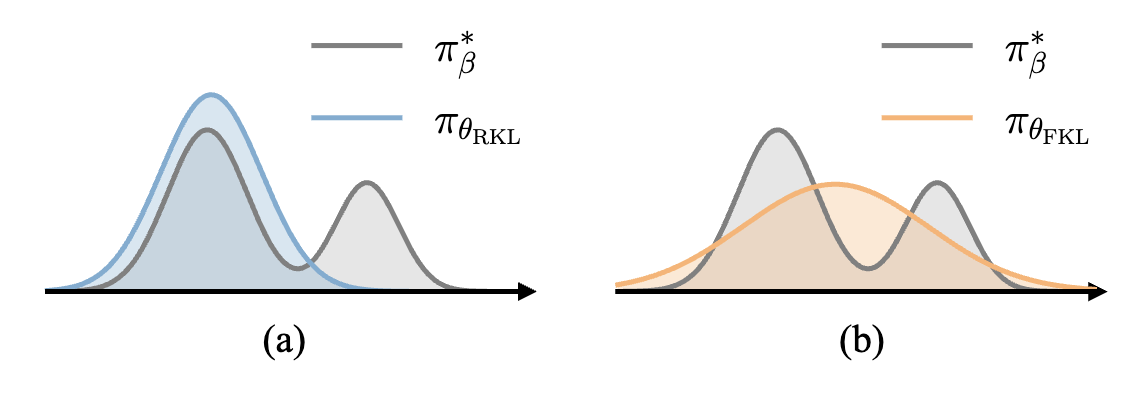
The above derivation shows how maximizing the reward in RL corresponds to minimizing the reverse KL divergence with a specific target distribution $\targetRL$ (since $\partition_{\targetRL}$ is a constant). This target distribution is the same as our standard sampling target $\target$ if we set $\potential(\sT) = e^{\beta r(\sT)}$! Though RL and TSMC have the same minimizer, they go for this with two different divergences: TSMC aims to minimize forward KL whereas RL aims to minimize reverse KL. Forward KL corresponds to covering the mass of the data distribution since you need to give nonzero likelihood to all samples. On the other hand, reverse KL encourages mode seeking behavior since you only care about the likelihood of samples generated under your own policies. This idea shows up a lot in generative modeling, with the following intuitive picture (Figure 1).
The typical way to optimize for this objective is via the policy gradient, which corresponds to the gradient of the expected rewards with respect to the generator policy; this is commonly implemented using REINFORCE or PPO. You may find this introduction to (off-policy) RL instructive to learn about how to optimize this objective (for both this section and the next section).
Soft RL (value-based)
Value-based RL comes from viewing the same KL-constrained RL problem with a different angle. Instead of taking the gradient with the expected rewards, valued-based RL finds a condition that the optimal policy must satisfy. It then optimizes this consistency loss.
We first define the soft value function for a given state $\st$ as
\begin{equation}\label{eq:value-marginal}V_t(\st) = \frac{1}{\beta} \log \sum_{s_{t+1:T}} \base(s_{t+1:T} | \st)e^{\beta r(\sT)}\end{equation}
where $V_T(\sT) = r(\sT)$ (this differs from the paper since we assume no intermediate rewards, or $r(\st) = 0$ for $t < T$). Intuitively, for a given state, this captures how much reward we expect to get if we sampled a trajectory from this state. We can also write this quantity recursively as
\begin{equation}\label{eq:value-bellman}e^{\beta V_t(\st)} = \sum_{s_{t+1}} \base(s_{t+1} | \st) e^{\beta V_{t+1}(s_{1:t+1})}\end{equation}
We can convert this into a consistency objective by ensuring that our estimates of the values are consistent with each other. This is called the soft Bellman operator and forms the basis of most value-based RL methods such as soft Q-learning (Haarnoja et al, 2018) and path consistency learning (Nachum et al, 2017).
Note that the conditions of the optimal twist look awfully similar to the conditions of the optimal value function: Equation \eqref{eq:twist-marginal} maps to \eqref{eq:value-marginal} and Equation \eqref{eq:twist-bellman} maps to \eqref{eq:value-bellman}. In fact, the twist function directly maps to the value function!
\begin{aligned} &\potential_T (\sT) = e^{\beta r_T(\sT)} &&r_T(\sT) = \frac{1}{\beta} \log \potential_T (\sT) \\ &\twist_t(\st) = e^{\beta V_t(\st)} &&V_t(\st) = \frac{1}{\beta} \log \twist_t (\st) \end{aligned}
Nice, twisting is actually just learning the value function (with a different divergence) in disguise! In the paper, the authors show that $\twist_t$ actually corresponds to the $Q$ function, which is defined as accepting an action $s_t$ via $Q_t(s_t, s_{1:t-1}) = V_t(\st) + r(s_{1:t})$. Since we are assuming there is no intermediate reward, we have that $Q_t(s_t, s_{1:t-1}) = V_t(\st)$ and we get to collapse their new notation $\Phi_t$ as equivalent to $\twist_t$.
Distributional RL
Can we fix the divergence of policy gradient and soft RL while retaining the benefits of maintaining a single policy? Minimizing the forward KL requires sampling from the ground truth distribution. If we had samples from the ground truth distribution, we could use them, and this corresponds to standard behavior cloning with cross entropy loss
\begin{aligned} &\nabla_\theta \KL{\target || q^\theta} \\ &=\nabla_\theta \Eof{\sT\sim \target}{\log \target(\sT) - \log q^\theta(\sT)} \\ &=\nabla_\theta \Eof{\sT\sim \target}{- \log q^\theta(\sT)} \\ &=\nabla_\theta H(\target, q^\theta) && \text{[cross entropy]} \end{aligned}
Unfortunately, we don't have sampling access to the base policy, and we might not have samples from the ground truth as well. Besides, isn't RL supposed to involve sampling from your current policy? We can remedy these issues by appling importance sampling to properly account for forward KL. This natural importance sampling method would correspond to
\begin{aligned} &\nabla_\theta \KL{\sigma || q^\theta} \\ &= \Eof{\sT \sim \target}{\nabla_\theta q^\theta(\sT)} \\ &= \Eof{\sT \sim q^\theta}{\frac{\sigma(\sT)}{q^\theta(\sT)}\nabla_\theta q^\theta(\sT)} \\ &= \Eof{\sT \sim q^\theta}{\frac{\unnorm{\sigma}(\sT)}{\partition_\sigma q^\theta(\sT)}\nabla_\theta q^\theta(\sT)} \\ \end{aligned}
which corresponds to standard importance sampling. There are a couple design decisions on how to approximate this expectation when drawing a batch of samples from proposal $q_\theta$. The first choice is whether to use self-normalized importance sampling (estimating your partition function from the batch). If using SNIS, the second choice is whether to apply the importance weights when resampling from the proposal batch or when computing the gradients. Regardless, the main idea of Distributional Policy Gradient (DPG) is to estimate this expectation via importance sampling from your policy. Unfortunately, your proposal distribution will often be high variance, making it difficult to apply this algorithm.
Partition function evaluation
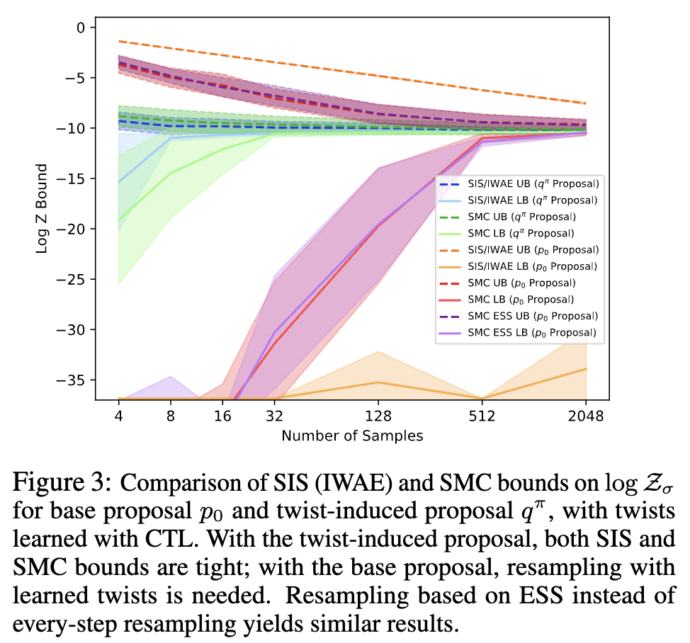
I will not go into depth here, but you can evaluate the quality of your sampling algorithm by how well it estimates the partition function. Namely, you can construct upper and lower bounds on the partition function with your chosen sampling weights. The paper claims that a good sampling algorithm would correspondingly have tight bounds on $\log \partition$, making it a good task to evaluate models on. In Figure 2, sampling using the twisted proposal $q^{\pi}$ results in really tight bounds on $\log \partition$ with few samples, implying that this provides a lot of variance reduction. One can evaluate the quality of simple importance sampling and SMC by comparing the tightness of the bounds equipped with a worse proposal (the base policy $\base$).
Conclusion
The paper discusses the connection between reinforcement learning and probabilistic inference, showing how one can approach the sampling problem either through learning proposals or learning twist functions. I didn't cover some other aspects such as conditional sampling and bidirectional Monte Carlo, please read the paper if you're interested. In general, I find these clever sampling algorithms quite cool, giving a lot of gains for very little problem structure. Thank you for reading, and feel free to reach out with any questions or thoughts!