Perturbation Invariant Gradients: Permutation Case Study
\( \def\R{\mathbb{R}} \def\wavg#1{\overline{f(x_{#1:T})}} \)5/16/2025
When given a limited number of data points, practitioners have found great success in creating synthetic samples by augmenting data with a known invariance. For example, in image classification tasks such as CIFAR-10, there has been great success in adding data augmentations such as Gaussian noise, random cropping, and horizontal flips. In language modeling, rephrasing and more sophisticated transformations have been used to create more realistic data from a seed corpus of "real" data (Maini et al, 2024 ; Yang et al, 2024).
In some cases, it is rather computationally expensive to both generate many augmentations and then train on them. For example, in Kotha et al, 2025 we find that you can train on up to 1000 rephrases from the student model with strong log-linear returns on downstream performance. However, it feels rather wasteful to generate so many augmentations when we have access to the form of the exact augmentation distribution and student model.
In this post, we question whether it's possible to "collapse" this into a simpler process. Instead of taking multiple steps on multiple draws of the distribution, we try to compute the expectation of the gradient over the perturbation distribution. We hope that in some cases (1) it's computationally easier to compute the expectation and (2) it contains more information than a small number of augmentations.
Since the general case is difficult (and potentially impossible), we focus on a simpler problem where it is feasible to computed the expected gradient: linear regression with permutation invariance. The expected gradient for this case ends up being cheaper to compute than standard augmentation. It both reduces the loss faster and has a better loss asymptotically compared to sampling augmentations.
Linear Regression with Permutation Invariance
Data
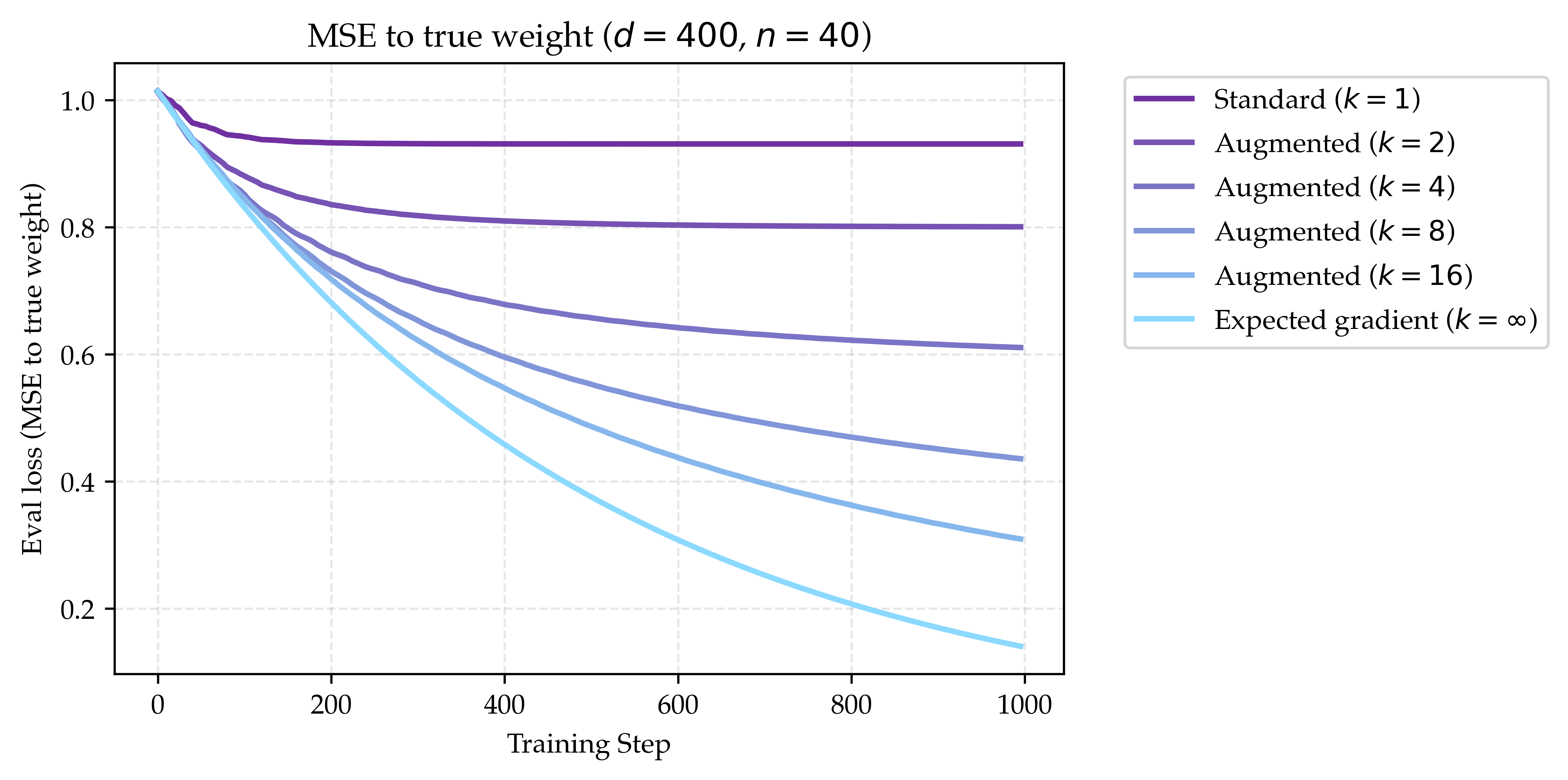
We will consider standard linear regression. In this problem, a ground truth $w^* \in \R^d$ governs a data distribution $\mathcal{D}$ of data points $(x, y)$, where $x \sim \mathcal{N}(0, I_d)$ and $y = w^{*\top} x$. We hope to learn the weight vector using $n$ samples from this distribution. We set $d=400$ and $n=40$ to represent a lack of data to fully recover $w^*$ in the general case.
Training
We will learn weight $w$ using stochastic gradient descent. Our goal is to minimize the mean squared error $\mathcal{L}$ of the predictor. We express this up to a constant factor as
\begin{aligned} \mathcal{L}(w) &= \frac{1}{2} \mathbb{E}_{(x, y) \sim \mathcal{D}} \left[\ell(w; x, y)\right] \\ &= \frac{1}{2}\mathbb{E}_{(x, y) \sim \mathcal{D}} \left[\left(w^{\top} x - y\right)^2\right] \end{aligned}
which is also proportional to $||w - w^*||_2^2$. We minimize this loss using stochastic gradient descent. At each training step, we take a single data point $(x_i, y_i)$ and take a gradient step to minimize mean squared error. The gradient is given by
\begin{aligned} \nabla \ell(w; x, y) = (w^{\top} x - y)x \end{aligned}
which gets scaled by the learning rate. When we run out of data points, we will start epoching over the data. We show the results of this training process as the highest purple curve in Figure 1. Since $n$ is much smaller than $d$, it is expected that the loss will stop improving after a certain point using standard gradient descent.
Invariance
In general, data augmentations are used when the training process is oblivious to some invariance of the true training distribution (i.e. image class is invariant to Gaussian noise). In our linear regression setting, we will add a strong invariance to the true weight $w^*$: every entry of $w^*$ is equal to each other. Leveraging this invariance is really important for generalization: without using it, there are $d=400$ degrees of freedom, whereas under the invariance there is only one. Without loss of generality, we can assume that $w^*$ is a vector of ones.
Setting all the entries equal to each other introduces a permutation invariance over the data distribution; namely, for any permutation $\pi(x)$ of true input $x$, we know that $(\pi(x), y)$ is also a valid data point. Unfortunately, standard training is oblivious to this invariance and will not be able to achieve low error.
We now introduce a simple data augmentation that captures this invariance: permute the input $x$ with random permutation(s) $\pi$. To mirror real settings, we will assume it is not free to both permute the data points or take the gradient step on the permuted data points. We now train as follows:
- For each data point, sample $k-1$ additional permutations for $k$ total points.
- For each gradient step, take the gradient on the $k$ points in one batch (i.e. train with batch size $k$ on augmentations).
- When data is exhausted, start epoching over the data.
The new gradient step can be interpreted as redefining the gradient of the loss $\nabla \ell(w; x, y)$ to be the average over the $k$ permutations. We show the results of this training process in Figure 1 for $k\in\{2, 4, 8, 16\}$. We note that as we increase the number of permutations, the loss decreases faster. However, under our current model of computation, this strategy costs $k$ times more compute for both synthetic data generation and training.
Expected Gradient
It feels rather wasteful to generate i.i.d. permutations and take gradient steps on them. We note that as $k\to\infty$, the gradient update approaches the expected gradient over the permutation distribution. We now explore the possibility of computing the expected gradient over the distribution of permutations. Namely, the infinite compute limit of our strategy would perform the following update:
\begin{aligned} \nabla \ell(w; x, y) := \mathbb{E}_{\pi} \left[\nabla \ell(w; \pi(x), y)\right] \end{aligned}
When we write the update as this infinite sample limit, the problem becomes more tractable. In fact, we can solve for the exact expected gradient as a function of $x, y$ and $w$. In Appendix A.1, we show that the $i$th entry of the expected gradient is given by
\begin{aligned} \frac{s_{x^2}}{d}w + \frac{\left((s_x)^2 - s_{x^2}\right)\left(s_w - w_i\right)}{d(d-1)} - \frac{ys_x}{d} \mathbf{1}_d \end{aligned}
where $s_x = \sum_{i\in[d]} x_i$, $s_{x^2} = \sum_{i\in[d]} x_i^2$, and $s_w = \sum_{i\in[d]} w_i$. Though this is kind of disgusting, it is actually simple to find this quantity as a function of $x, y, w$ and only takes a small constant factor longer than computing the standard gradient. We show the loss when taking this expected gradient step as the lowest blue curve in Figure 1. Not only is it cheaper to compute, but it learns faster matched on a step-for-step basis and has a smaller plateauing loss than small $k$. This shows that the expected gradient is a helpful operator for this specific problem.
Next steps
The above derivation required a lot of structure over the model and data distribution. I see two approaches to continue pushing this forward
Bottom-up approach: Gaussian perturbations
I think a reasonable way to make some progress is to slowly generalize this to more non-trivial models and augmentation strategies. For example, we could consider the case where we want to compute the expected gradient over Gaussian perturbations. Unfortunately, I ran into some trouble doing this even for simple multi-layer linear models. At a high-level, I took the approach of using $\mu$P-style arguments, specifically the Gradient Independence Assumption (Schoenholz et al, 2017 ; Yang, 2022). Unfortunately, I under-appreciated how important it is that standard backpropagation is a rank 1 update to the weight vectors. For the expected gradient, you need to track both the mean and the covariance matrix of each intermediate layer. This is prohibitively memory and compute intensive for wide models, taking one from compute linear in hidden size (due to rank 1 updates decomposing into vector-vector products) to quadratic. I do not know if this is a fundamental issue or if it is resolvable by the correct assumption on the structure of the noise. I am being vague and lazy here so please reach out if I can expand on this for you.
Top-down approach: Rephrasing
The actual target application I am most interested in is rephrasing. In this setting, we have a known invariance over the data distribution. The main departure from the traditional augmentation setting is that it is parameterized by model parameters. In fact, as we discuss in a previous blog post, this set of parameters can be the same as the student model. In this setting, it feels extra wasteful to do the generation and training seperately. I wonder if there is a way to collapse this process into a simpler step considering that we have the exact parameterization of the distribution of interest. Also reach out if you have thoughts on this.
Conclusion
Data augmentation is a powerful tool for leveraging invariances in data unknown to the training process. Hopefully, we can make it more scalable by leveraging structure in the augmentation distribution, like we can for permutation invariance. Thank you for reading, and feel free to reach out with any questions or thoughts!
Assets
You can find the code for the plot in Figure 1 at this repository. Most of this code, math, and experiments were done in one long ChatGPT conversation, as well as light modifications in Cursor. For pedagogical purposes, I'm sharing the (relatively embarassing) ChatGPT conversation.
Appendix
A.1: Computing the expected permutation gradient
As a quick refresher, the standard gradient for our loss is given by
\begin{aligned} \nabla \ell(w; x, y) = (w^{\top} x - y)x \end{aligned}
Now, we can try solving for the expected gradient over the distribution of permutations.
\begin{aligned} &\mathbb{E}_{\pi} \left[\nabla \ell(w; \pi(x), y)\right] \\ =\;& \mathbb{E}_{\pi} \left[(w^{\top} \pi(x) - y)\pi(x)\right] \\ =\;& \mathbb{E}_{\pi} \left[(w^{\top} \pi(x))\pi(x)\right] - y\mathbb{E}_{\pi} \left[\pi(x)\right] \\ \end{aligned}
For convenience, we will define the following terms
- The sum of entries of $x$ as $s_x = \sum_{i\in[d]} x_i$
- The sum of the squares of the entries of $x$ as $s_{x^2} = \sum_{i\in[d]} x_i^2$
- The sum of the entries of $w$ as $s_w = \sum_{i\in[d]} w_i$
For the second term, since the expectation of the mean permutation is simply the vector of the average $x$ entry, it is given by
\begin{aligned} y\mathbb{E}_{\pi} \left[\pi(x)\right] = \frac{ys_x}{d} \mathbf{1}_d \end{aligned}
The first term is slightly more involved. We can first rewrite the $i$th entry of the gradient as
\begin{aligned} &\left(\mathbb{E}_{\pi} \left[(w^{\top} \pi(x))\pi(x)\right]\right)_i \\ =\;& \mathbb{E}_{\pi} \left[\left(\sum_{j\in[d]}w_jx_{\pi(j)}\right)x_{\pi(i)}\right] \\ =\;& \sum_{j\in[d]} w_j \mathbb{E}_{\pi} \left[x_{\pi(j)}x_{\pi(i)}\right] \\ \end{aligned}
Since this is a permutation, we can not assume $\pi(i)$ and $\pi(j)$ are independent and split the expectation. Instead, we can condition on when they are equal.
- When $\pi(i) = \pi(j)$, the inner expectation simplifies as $\frac{1}{d}\sum_{p\in[d]} x_p^2 = \frac{s_{x^2}}{d}$
- When $\pi(i) \neq \pi(j)$, the inner expectation simplifies as $\frac{\sum_{p\neq q} x_px_q}{d(d-1)} = \frac{(s_x)^2 - s_{x^2}}{d(d-1)}$
With this in hand, we can write the full summation as
\begin{aligned} & \sum_{j\in[d]} w_j \mathbb{E}_{\pi} \left[x_{\pi(j)}x_{\pi(i)}\right] \\ =\;& w_i \frac{s_{x^2}}{d} + \sum_{j\neq i} w_j \frac{(s_x)^2 - s_{x^2}}{d(d-1)} \\ =\;& w_i \frac{s_{x^2}}{d} + \frac{\left((s_x)^2 - s_{x^2}\right)\left(s_w - w_i\right)}{d(d-1)} \\ \end{aligned}
Putting it all together, we get that the $i$th entry of the full expected gradient $\mathbb{E}_{\pi} \left[\nabla \ell(w; \pi(x), y)_i\right]$ is given by
\begin{aligned} \boxed{\frac{s_{x^2}}{d}w + \frac{\left((s_x)^2 - s_{x^2}\right)\left(s_w - w_i\right)}{d(d-1)} - \frac{ys_x}{d} \mathbf{1}_d} \end{aligned}
Though this is truly a disgusting expression, the main point is that it's a simple function of the entries of $x, y$ and $w$ and doesn't depend on the permutation $\pi$. We could probably simplify it drastically if we assumed that $\pi(x)$ was a random sample with replacement, which is a simple approximation.